


ABSTRACT
This article discusses the use of predictive analytics in asset management. It starts by defining predictive analytics and explaining how it differs from business intelligence and artificial intelligence. The stages in carrying out analytics projects are then discussed with reference to the CRISP-DM process. Particular emphasis is placed on having a clear understanding of the business objectives of the project, becoming familiar with the data, and using the appropriate model to develop a solution that is credible, solves the business problem and can be implemented. Such a solution can help organisations gain insight and understanding into the causes of asset failure and so improve their operational and financial performance.
The advantages of modelling asset failure in the time domain rather than only using static factors are then discussed. A case study from the water industry is used to show how advanced predictive analytics (Cox regression and Kaplan Meier risk curves) can be used to model asset failure in the time domain and so optimise asset management at individual asset level and at the operational, tactical and strategic levels.
Introduction
More and more organisations are realising the hidden value of the data they hold on all aspects of their business, including the performance of their assets. This requires them to acknowledge two things: firstly, that data are an asset to be exploited for improving the performance of the organisation; and secondly that predictive analytics is the means by which this objective can be achieved.
Developing predictive analytics models requires knowledge and experience. Before the models can be developed, the data must be prepared − a process that cannot be automated because of the infinite number of data issues that can be present and must be considered. Only after all the necessary data preparation procedures have been developed can the models be developed and then run automatically. However, the software can only deal with data issues that it explicitly addresses. It cannot address other data issues and models based on incorrect data will lead to invalid results.
The analytics must always be applied in a structured and rigorous way if they are to improve the quality and validity of business decisions and so be of value to the organisation. The benefits of applying predictive analytics are more achievable now than ever before because of the increasing amount of data, ready availability of software and powerful hardware. However, analytics alone is not the answer to how to gain business advantage from the ever-increasing amount of data and low cost of computing power. Rather, the answer consists of a number of steps:
- understanding the business problem
- working out the data required
- identifying what data are available
- designing and building a credible and practical solution to the business problem that uses available data and appropriate analytics; and
- implementing the solution.
These steps are a summary of the CRISP-DM process (see ‘Developing Predictive Analytics Models’ below).
The ready availability of easy to use software (including black-box software, in which the user has no knowledge of how the input data are transformed to the output data) does not detract at all from the importance of understanding the data, preparing them correctly and using an appropriate model that is understood and whose assumptions and limitations are known. Predictive analytics that uses incorrect data, incorrectly prepared data or unsuitable models will not address the business problem and so may lead to inappropriate and costly decisions and actions being taken.
The difference between predictive analytics and business intelligence
The term “predictive analytics” is widely used but unfortunately not well understood. The reasons for this are unclear, and so it is best to start by defining these terms and the term ‘business intelligence’.
Predictive analytics is the branch of advanced analytics that is used to make forecasts and predictions about the outcomes of a range of scenarios using models developed from historical data. It uses techniques from data mining, statistics, machine learning and artificial intelligence, and is used in many sectors of the economy, including infrastructure asset management (the subject of this article), process control, fraud detection, passenger demand forecasting and sales forecasting. Examples predictive analytics models are regression, decision trees and time series models.
Business intelligence is another term that requires clarification because it is often used synonymously with predictive analytics, whereas they are quite different and so should not be confused. The key difference between business intelligence and predictive analytics is their time horizons. BI looks backwards to report what has happened but does not provide any lessons from this history as to what may happen in the future whereas predictive analytics uses historical data to develop predictive models for reporting what is likely to happen under a range of different scenarios. Thus another difference between BI and predictive analysis is that BI only involves empirical analysis of data and does not require model development. The empirical analysis used in BI is at aggregated levels rather than at individual object level. On the other hand, predictive analytics works at the lowest unit of measurement and so is able to provide deep and meaningful insight, and identify objects that show unusual or unexpected behaviour.
Developing predictive analytics models
Developing predictive analytics models is much more work than putting together a few standard procedures. Before any data preparation work can start, the source data may have a range of problems that must be addressed. Typical problems include:
- Data may be stored in a variety of legacy systems and databases that cannot be read easily, or in silo spreadsheets (spreadsheets are not databases). Furthermore, a common problem with silo spreadsheets is that since they are owned by individual people (by definition) and not shared with other people, they tend to be poorly documented and have their own data definitions and formats, etc, so making them difficult to understand and link to other files
- the data were not recorded properly or at all
- transcription errors. They can be particularly problematic with data that were recorded manually
- data are not sufficiently granular
- inconsistent data
- duplicate records
- duplicate fields
- values for the same fields in different files with different definitions
- missing data
- very old data may not be relevant to current assets or operational procedures.
Only after these and similar problems have been addressed can the data be explored and prepared, and model development then begun. Throwing all the data into a model straight away without doing all the necessary preliminary work is akin to throwing the kitchen sink at a problem. It is not a viable strategy and will lead to spurious and unintelligible models.
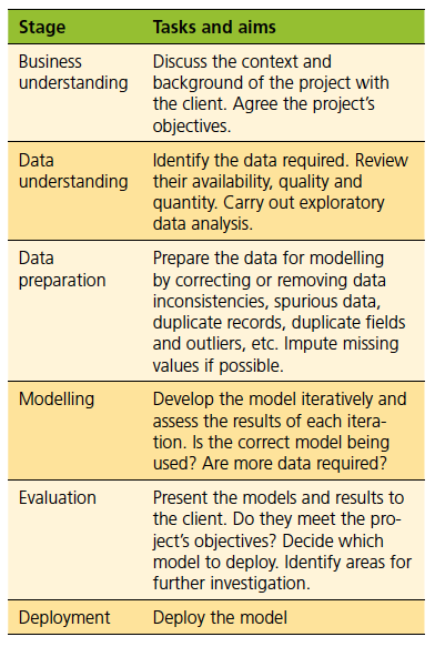
A common methodology for developing predictive analytics models is CRISP-DM (CRoss Industry Standard Process for Data Mining). It was conceived in 1996 by DaimlerChrysler, SPSS and NCR as a structured and robust methodology for planning and carrying out data mining projects. Figure 1 shows the six stages of CRISP-DM and its iterative nature.
CRISP-DM is iterative because the results of some stages may require the project cycle to go back to earlier stages. For example, a result of the modelling stage may be that more data preparation is required − new data may be needed or the existing data may have to be prepared in a different way. Each stage of the process is described in Table 1.
Proactive maintenance based on predictive analytics
A purely proactive maintenance policy is the ideal policy but is unachievable, because assets will always fail unexpectedly however good the maintenance policy and so require reactive maintenance. A proactive maintenance policy based on predictive analytics to determine which assets should be scheduled for maintenance should be the aim. This approach will not remove totally the need for reactive maintenance but it will minimise the occurrence of reactive failures. The minimisation is subject to operational and other constraints, for example the organisation’s maintenance capacity and attitude to the risk of asset failure.
Figure 2 summarises the trade-off between proactive maintenance and reactive maintenance. The key difference between them is that reactive maintenance asks questions about the past whereas proactive maintenance asks questions about the future.
A proactive maintenance policy based on predictive analytics has the following features:
- the maintenance schedule can be prioritised by the risk of failure or measures based on the risk of failure
- it minimises the total cost of asset management
- it establishes the factors that contribute to asset failure, so providing insight and understanding of asset failure
- the consequent costs of asset failure, for example flooding and pollution, are minimised.
Predictive analytics applied to asset management
Most current asset management systems are based on business intelligence and so do not have predictive functionality. As discussed above, business intelligence is concerned with presenting historical data, usually in aggregated form, using graphs and tables whereas predictive analytics reports what is likely to happen in the future in a range of different scenarios. The objective of predictive analytics is clear, but developing predictive models is not an insignificant task. Difficulties that may occur when developing models for predicting asset failure include:
- the causes of asset failure are many and varied, and so a wide range of data is required
- considerable domain knowledge and business understanding are required
- there may be insufficient historical data. Since asset failure occurs infrequently, the historical data must have enough failures for the model to extract the drivers of failure.
- asset failure models use advanced analytics and so experience and knowledge are required to develop them
- there may be complex interactions between the predictors in the model
- time dependent systems are in general more complex than static systems. Since the risk of asset failure changes as assets are used and maintained, asset failure should be modelled as a temporal phenomenon rather than only using predictors that do not change over time, for example the assets’ design specifications.
Implementing a new proactive asset management system based on predictive analytics is a major undertaking that needs careful and detailed planning (a subject outside the scope of this article). Two obstacles that may be encountered when implementing such a system are fear of the unknown and a reluctance to change. These feelings can be overcome by working with the people affected on a carefully designed programme that helps them gain an appreciation and understanding of why the changes are necessary for the good of the whole organisation.
Predictive analytics can answer a range of asset management questions, including:
- which factors contribute to asset failure
- how to optimise asset management at individual asset level and at the operational, tactical and strategic levels
- how does the risk of an asset failing change as it is used and maintained
- how does proactive maintenance affect the risk of subsequent asset failure
- how does repeated asset failure affect the risk of subsequent asset failure
- how does asset criticality determine which assets to maintain
- what is the effect of standby assets on asset group reliability.
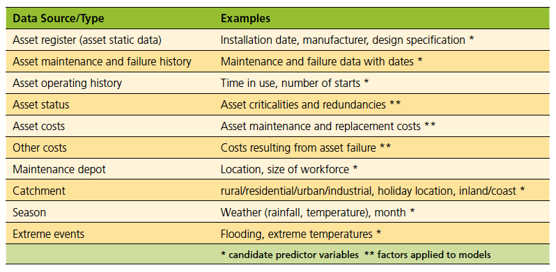
The data required for applying predictive analytics to asset management depend on the industry, organisation and asset type, and can be split into four categories: asset register data; asset maintenance and failure history data; other asset data; and external data. Table 2 shows example data for a range of asset types. It is unlikely that all the data in the table will always be available or required. Similarly, other data may be available or required.
Asset failure models
Regression is a statistical method for establishing the relationship between one variable (the target variable) and at least one predictor variable. The regression model is then used to estimate or predict values of the target variable from given values of the predictor variable(s).
The rest of this article will describe how the author has applied one type of regression model to asset failure. However, it is first worthwhile to explain very briefly why two popular types of regression model, linear regression and logistic regression, are inappropriate for modelling asset failure.
There are many types of regression model, ranging from linear models to the advanced models used in survival analysis. Linear models should not be used for modelling asset failure because they can easily predict negative values for target variables that can only take positive values, for example failure rate. Logistic models have binary target variables, for example failure/non-failure, and do not have this problem because the output is the probability of the event occurring. However, since time cannot be a predictor variable in logistic regression models, the calculated failure probabilities do not change over time as the assets are used. This is not realistic because the risk of asset failure increases with asset use (assuming there were no maintenance interventions).
Survival analysis is a class of statistical method for analysing and modelling the occurrence and timing of events, for example asset failure. In engineering it is sometimes called reliability analysis. With respect to asset management, survival analysis answers questions such as what is the probability of an asset surviving beyond a particular time and how do different factors contribute to asset failure.
Survival analysis regression models, for example the Cox proportional hazards model, overcome the problems described above because time is an intrinsic part of the models. They model the risk of asset failure as a dynamic phenomenon where the output is a probability of failure of each asset at each sampled time and so the model can be used to predict the risk of assets failing as they are used. The Cox model can be used to model the relationship between failure rate and a number of predictors.
In some ways, the Cox proportional hazards model can be thought of as logistic regression in the time domain. Since the model also includes static factors such as those in Table 2, it can provide insight and understanding into the causes of asset failure.
Survival analysis modelling
When applied to asset management, because it is a predictive model in the time domain Cox regression can be used to identify and monitor individual assets, and model the following conditions:
- repairable and non-repairable assets
- asset redundancy
- measures of the risk of asset failure
- asset management optimisation.
Identifying and monitoring individual assets
Most if not all current asset management systems only use static categorical data, for example manufacturer and design specification, to describe the assets. It is very unlikely that such a classification system can define assets uniquely because at least two assets can have the same factor values. Consider the case of three factors used to describe the assets (the number in brackets is the number of categories for the factor): manufacturer (2); power (3); and location (4). If only these factors are used, there are 24 value combinations. If the number of assets is smaller than 24 and the assets have different value combinations, the assets can be defined uniquely; but if at least two assets have the same value combination, the assets cannot be defined uniquely. However, if there are at least 25 assets, some combination will occur at least twice, and so it is impossible to identify each asset uniquely using only these factors.
Even if some assets are identical with respect to their static factors, they will almost certainly have different maintenance and failure histories. It is this additional time dependent information that differentiates the assets and can be used in survival analysis regression models to identify and monitor each asset as a unique entity if the data are in the correct form in the model.
Repairable and non-repairable assets
A repairable asset is an asset that can be restored to a state in which it functions satisfactorily, if not to its original state. A non-repairable asset is an asset that is replaced at first failure. These assets tend to be cheaper than repairable assets and not critical. The models for non-repairable assets are simpler than the models for repairable assets because they only have proactive maintenance and are replaced after their first failure, whereas repairable assets have proactive and reactive maintenance.
Asset redundancy
The redundancy of a group of assets is the survival probability of the group when the number of assets available is greater than the number of assets required. It is calculated from the survival probability of each asset in the group, the number of assets that are required and the number of assets that are available, and is modelled as a probability by applying probability theory to the survival probabilities.
As an example, consider three assets with survival probabilities 0.6, 0.7 and 0.8. If one asset is required at all times so that at least one asset must be available, it can be shown that the redundancy is 0.976. This means that at least one asset will be available on average 97.6% of the time. If two assets are required at all times, the redundancy is 0.788. Thus, at least two asset will be available on average 78.8% of the time. The redundancy does not matter which asset are in use − it is the survival probabilities of the assets in the group that define the group redundancy.
Measures of the risk of asset failure
The risk of failure for each asset can be measured in a number of ways, including the:
- probability of the asset failing at time t
- probability of the asset failing at time t adjusted by all the costs resulting from the asset’s failure (the costs of intervention and asset replacement, and the consequent costs of failure)
- probability of the asset failing at time t adjusted by the asset’s criticality.
The first measure is the output of the asset survival model. The second and third measures weight this probability by each asset’s costs of failure and criticality respectively. Thus, it is possible that a critical asset with a low probability of failure has a higher risk of failure than a moderately critical asset with a medium probability of failure. Each risk measure for each asset can be calculated and a prioritised list of assets for maintenance can then be drawn up by ranking the assets in each list and using the ranks and domain knowledge to combine the three lists into a ranked asset maintenance list.
Asset management optimisation
The asset management policy can be optimised at individual asset level (discussed above), and at the operational, tactical and strategic levels.
Operational level asset management optimisation identifies assets at greatest risk of imminent failure so that they can have proactive maintenance to reduce their risks of failure rather than be repaired or replaced after they fail, and also be maintained rather than assets that are scheduled for maintenance then but whose risks of failure then are smaller. This allows a virtuous proactive maintenance feedback policy to be created.
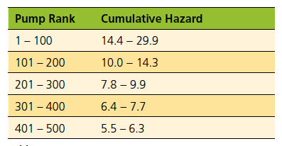
Figure 3 shows the distribution of cumulative hazards for 8,500 clean water and waste water pumps in 800 locations (cumulative hazard, the integral of the hazard rate with respect to time, is a measure of the accumulated risk of failure for an individual asset as it progresses along the failure rate curve towards failure). The pumps are ranked in descending order of their cumulative hazards (risk of failure) at a given time (pump rank 1 has the highest cumulative hazard and pump rank 8,500 has the lowest cumulative hazard). The distribution is highly skewed − a very steep decrease followed by a long tail.
Table 3 summarises the cumulative hazards of the 500 pumps in greatest need of proactive maintenance (pump ranks 1 to 500) in Figure 3. It shows that the range of the 100 largest cumulative hazards is 15.5. This is about half the range of all the cumulative hazards but is accounted for by only 1.17% of the pumps. As with Figure 3, Table 3 clearly shows the highly skewed distribution of the cumulative hazards.
Tactical level asset management optimisation involves producing a series of deterioration (risk) curves that show how the risk of asset failure changes for different values of a factor, for example manufacturer, as the assets are used. The curves identify the asset type with the highest survival probabilities (or lowest cumulative hazards).
Figure 4 shows the cumulative hazard curves for 2,250 pumps in waste water pumping stations for four manufacturers in 800 locations. The curves consist of a series of discrete points where each point is an asset, rather than being continuous. At all times pumps from manufacturer D had the highest cumulative hazards (risks of failure) and pumps from manufacturer A had the lowest cumulative hazards, and so pumps from manufacturer A had the lowest maintenance costs. After ten years, the risk of failure of pumps from manufacturer D is about 3.25 times that of pumps from manufacturer A (1.3/0.4).
The small crosses on the graphs are censored assets. Censored assets are assets that did not fail during the study. Censoring is an important concept in survival analysis. It is used to account for assets that had not failed by the end of the study − this does not mean that they will never fail, only that their failure was not observed during the study.
Strategic level asset management optimisation requires simulating the financial implications each month of a range of asset maintenance and replacement policies to work out the optimal, i.e. most cost-effective, policies subject to a range of factors, for example the organisation’s maintenance capacity and attitude to the risk of asset failure.
Figures 5, 6 and 7 show simulation results for 2,250 pumps in waste water pumping stations in 800 locations where maintenance capacity is a constraint and is respectively 20, 60 and 100 interventions a month. The results are the pumps’ maintenance and replacement costs for the next five years (the consequent costs of asset failure are not included). The figures show how the penalty (the pumps’ maintenance and replacement costs) varies with the percentage of proactive interventions (the percentage of interventions that are proactive as opposed to reactive) for each risk tolerance (the maximum acceptable level of repeated asset failure an asset can have before it is replaced). It is measured on a five-point scale, ranging from risk averse (1) to risk tolerant (5).
In analysing Figures 5, 6 and 7, it is important to note that risk tolerant asset management policies can lead to very high consequent costs. Since these costs are not included in the penalty figures, the total cost of risk tolerant polices can be significantly greater than the costs shown in the figures. Risk averse policies can also lead to consequent costs but they are likely to be smaller than the consequent costs of risk tolerant policies.
All the figures show that the penalties of maintenance policies that consist only of reactive maintenance are much greater than the penalties of maintenance policies that are proactive, even to a small extent. They show that for all risk tolerances the penalty decreases as the proportion of proactive maintenance increases, except at high maintenance capacities and very risk tolerant policies, the extent of the decrease depending on the maintenance capacity. At very high percentages of proactive intervention, high maintenance capacities and risk tolerant policies (orange diamonds in Figure 7) the curve flattens out, reaches a minimum, i.e. the optimal point, and then starts to rise very slowly. Too much maintenance is being carried out and the costs increase beyond the optimal point.
If the optimal asset management policy is the policy that minimises the assets’ maintenance and replacement costs, Figures 3, 4 and 5 show that (consequent costs are not considered):
- If the maintenance capacity of the organisation is very low, the optimal asset management policy cannot be achieved.
- If the maintenance capacity of the organisation is very high, at high risk tolerances and in the limiting case of exclusively proactive or almost exclusively proactive maintenance the penalty increases slightly from its minimum value. In this case the optimal asset management policy does not require all the maintenance capacity. If all the capacity is used, unnecessary costs due to excessive maintenance will be incurred.
- For all other maintenance capacities, the optimal asset management policy is achieved at high levels of proactive maintenance. The reduction in the penalty becomes progressively smaller as the level of proactive maintenance increases. When other costs, such as lower consequent costs associated with high levels of proactive maintenance, are included the curves become steeper and then flatten out, making the optimal point or region clearer.
Conclusion
Developing predictive analytics models is not a recipe-driven linear process. Rather, it is an iterative process that involves business understanding, data understanding, and knowledge and understanding of analytics − all three components are essential for a practical solution to the business problem to be produced. It is not uncommon for stages prior to model development to take about 75% of a project’s time so that when model development begins the basic structure of the model has been established, if only approximately.
Predictive analytics is a step beyond business intelligence because it requires deeper skills and greater effort. The additional effort is time well spent because predictive analytics can generate valuable insight into asset failure and so help mitigate the risk of future asset failure, something that business intelligence cannot do. In summary, unlike business intelligence, predictive analytics can answer two fundamental questions: why and how.
The potential savings of applying predictive analytics to asset management are very great because the costs of asset failure can be large and extend beyond the direct costs of asset maintenance, repair or replacement. For example, in the water industry the consequent costs of asset failure can be many times the cost of repairing or replacing the asset. Since consequent costs decrease as the proportion of proactive maintenance increases, the total cost of asset failure can be reduced by adopting a more proactive maintenance policy − even a small increase in the proportion of proactive maintenance can generate big savings. Predictive analytics can help increase the proportion of proactive maintenance but it cannot guarantee the elimination of unexpected failures. Rather, it can help minimise the requirement for reactive maintenance and thereby reduce the total cost of asset failure.

Dr Atai Winkler
Atai Winkler is an experienced predictive analytics consultant, and founder of PAM Analytics.
www.pamanalytics.com