

ABSTRACT
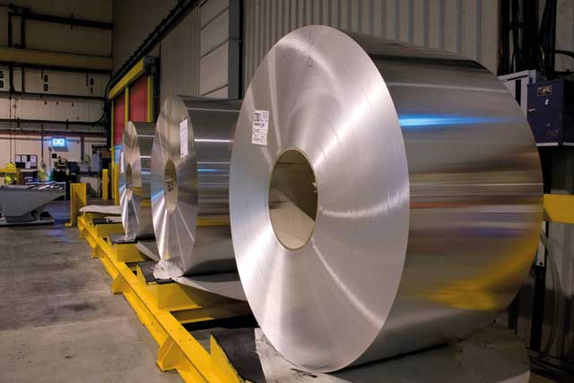
The Agfa Graphics Ltd plant in Leeds ran two continuous process lines (24 hrs Å~ 7 days) electrochemically treating aluminium to produce substrate for lithographic printing plates. These aluminium reels were typically 1,000 mm wide Å~ 0.275 mm thick, weighing 6 tonnes (Fig 1).
With a worldwide network of plants and a slowly declining sales volume due to technology shifts in the market, there was intense internal competition between the companies’ factories worldwide, because product loading was biased towards the most efficient plants. The Leeds plant adopted the strategy of focusing on reduced consumption to reduce manufacturing costs. Particularly noteworthy successes were achieved with gas, electricity, water, and acid consumption reduction and a move from 6,000 tonnes of general waste to landfill to zero tonnes. Collectively, this type of work won the IMechE MX awards for sustainable manufacturing in 2007 and 2011.
This article will focus on the way energy consumption was characterised and then reduced using classic continuous improvement (CI) techniques (Demings PDCA or the more modern Six Sigma DMAIC processes). This approach was followed because there was already a strong culture of CI in the plant and because capital was severely restricted given the business environment. The specifics of what was done in the Leeds plant may not be directly transferrable to other businesses, but the processes followed should be illuminating to others.
Understanding the split of gas consumption
At the start of the project in late 2005 there was an objective to reduce gas consumption, but the only data available was the annual gas consumption of around 9,500 MWh. Quotes were obtained to fit sub gas meters at various points in the site to understand how and where the gas was consumed. However, because it was not known whether consumption could be reduced, the capital costs quoted to install meters with hard-wired connections to the site systems were considered much too high, with uncertain payback.
The team came up with an imaginative solution to the problem, which was to get the security guard on his nightly rounds to read the single main incoming gas meter and enter the results in a spreadsheet on the site server.
The chart (Fig 2) shows the resulting picture over a two-year period. The peaks are the winter months, and the troughs are the summer months.
The data obtained was very variable from day to day. This noise was inspected and correlated with what was happening at the time of the reading: for example the drop to zero in the middle of the chart is a summer shutdown of one line followed by the other. By knowing when one line or the other was down for extended maintenance, overhaul, breakdown or product change, the basic split of the gas consumption was identified by comparing days with full production from a line and days with zero production from a line.
The results were: Line 1 consumed around 11,700 kWh/day when in full production; line 2 consumed around 7,300 kWh/day when in full production, and the balance was space heating ranging from 17,500 kWh/day in winter down to close to zero in the summer.
The consumption on both production lines was from a gas boiler heating a pumped circulating pressurised hot water system to heat process baths via plate heat exchangers. The major consumer of heat on both lines was the final wash system, where a continuous flow of deionised water was heated up from ambient (circa 12ÆC) to 50ÆC to wash the aluminium “photographically” clean. This was a one-pass system requiring continuous high heat input.
Other ways of heating this flow were investigated but none was as efficient (cheap) as the existing system.
A parallel project provides inspiration
Many improvement projects were under way in the factory at the time, including one to increase the capacity of the production lines. One capacity bottleneck was removal of heat from the electrochemical cells on the lines. In these cells high currents were passed through acid solutions to the aluminium to transform the aluminium surface. One of these processes was the anodising process. DC current heated up the sulphuric acid in the cells via Ohmic heating, in which the heating is proportional to the current squared multiplied by the resistance in the cell (iÇr). Several thousand amps were passing through four cells on the larger of the two lines. The heat was removed from the acid via plate heat exchangers, with coolant being pumped through being sent to an evaporative cooling tower for cooling before being pumped back.
In order to investigate the cooling capacity constraint (during summer months with higher temperatures and humidity making the cooling tower less effective) the team had constructed a view of the whole cooling system on the process control system (Fig 3).
The important figure on this screenshot is highlighted in the green box. At this moment the cooling tower is removing 2.015 MW of heat.
The link was made that on the same line we needed to find a heat source, for the final wash system in order to reduce gas consumption, and a heat sink, to take load away from the cooling tower for the electrochemical systems.
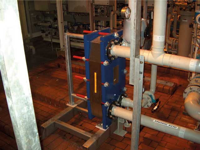
In spring 2007 a solution was designed, costed and fitted that took the hot acid from the anoidising process through one side of a new plate heat exchanger and the cold deionised water for the wash process through the other side (Fig 4).
The new scheme dramatically reduced the gas consumption on line 1 from around 11,700 kWh/day to around 3,500 kWh/day.
The cost of the installation (shown in Fig 5) was í26,000; in the first 12 months í65,000 worth of gas was saved.
However, the implementation had some problems. Insufficient thought had been given to non-standard operating conditions. It was found that when the anodic power was reduced or turned off, the waste heat recovery continued to cool the anodic acid, creating start-up problems getting the process back within temperature specification.
These problems were resolved by fitting automatic valves controlled by the main control system to shut off the cooling when the anodic system was not creating heat.
It is worth noting that the production team quite reasonably wanted to ditch the new system when the first problems with low anodic temperature were encountered because significant waste was being caused. It was important that the plant manager could see the end state and insisted that the system was fully adopted following the modifications.
Next steps for gas reduction
Once new the line 1 system was fully proven, a repeat project was carried out on line 2 in summer 2008, and this successfully reduced line 2’s consumption from around 7,300 kWh/day to 2,300 kWh/day.
The cooling tower was still required at the end of these projects. All of the heat from the anodic systems was not removed by the wash water and none of the heat from the other electrochemical systems (graining) was removed. However, the cooling tower then had some extra capacity due to this work and coped better on hot, humid days.
With both projects done, the space heating was the main remaining consumer of gas. Gas was being consumed in three areas. The first was the offices, where a few small gas boilers fed a hot water system going to radiators to provide heating. The second was around the warehouse/storage areas of the factory where there were seven gas burning air heaters. Finally in the production area was a heating ventilating & air conditioning (HVAC) unit, which produced temperature-controlled very clean air to the production lines.
The following was done to subdivide and understand the heating consumption. First, the offices were only heated on Monday to Friday. The gas consumption for heating at the weekend was compared with midweek, and the office consumption was inferred from the difference (around 7% of the space heating gas).
The gas space heaters in the warehouse had a fan motor and a burner assembly and were either fully on or fully off, controlled by thermostat. The site electrician suggested fitting a í10 run timer to each fan motor (see Fig 6).
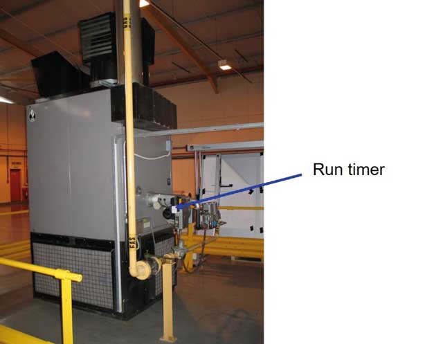
The fan motor only came on when the burner was on, and the capacity of the burner was fixed and known. Therefore, by knowing how long the fan had been running in a day the gas the space heater had consumed could readily be calculated.
Each of the seven space heaters’ run timers were added to the security guard’s daily walkaround and the results placed in a spreadsheet. In this way the gas used to heat the warehouse was found to be around 29% of the total space heating gas.
Knowing the office and warehouse consumption allowed the production area consumption to be estimated, at around 64% of the space heating. This was the area that was looked into further.
Reduction of production area space heating gas consumption
The HVAC system consisted of air being drawn through filters, across a large cooling coil and across a smaller heating coil. The cooling coil was fed by a chiller, but was inactive most of the year because Leeds rarely gets warm enough to require it (the air temperature specification for the production area was a maximum of 25ÆC). The heating coil was fed by a gas boiler providing circulating hot water. The heating coil was used most of the year.
Beneficially for the project, the HVAC unit was situated adjacent to the cooling tower referred to earlier. The proximity allowed the installation of another heat exchanger which, in all but the hottest two or three months of the year, would have the coolant from the HVAC cooling coil diverted to it which would be heated by the cooling tower return water.
In Fig 7 (below), HX is the new heat exchanger. Water returns to the cooling tower at around 28ÆC from the process line and is fed to the cooling coil circuit for the HVAC system via HX.
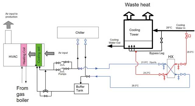
The HVAC cooling coil then instead becomes a pre-heating coil for air for the production area with liquid at 26ÆC within it.
Because the cooling coil had a very large surface area it became a very efficient pre-heater, and the gas heated heating coil only came into use when the external air went below 5ÆC.
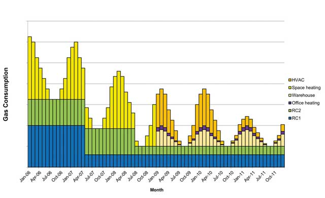
Fig 8 shows the smoothed monthly gas consumption from Jan 2006 to December 2011, clearly showing the impact of the line 1 project in May 2007, the line 2 project in July 2008, and the HVAC project in September 2010.
Electricity consumption reduction
Encouraged by the early successes with gas reduction it was decided to investigate what might be possible for electricity reduction, with the project commencing in 2010. Work had been done prior to this project, replacing old lights with more modern efficient ones, with sensors to turn lights off when nobody was present. However, although significant energy was saved, on a site level this was not significant.
What had never been done before was to look at the electrochemical process lines where most of the electrical energy was consumed. For the decades before this project, this usage was considered fundamental to the product and thought to offer no opportunities.
Being a large consumer (at the time the plant consumed 28,000 MWh of electricity annually at a cost of just over í2,000,000), the team had access to half hourly meter readings from the supplier.
Note that sites which consume more than 100,000 kWh of electricity per annum will have a half hourly meter. This data had never been examined before. Fig 9 is an example from June 2010 for the Leeds site.
At this time there were two distinct product types being produced which had different specifications for surface roughness and anodic weight. This required different current flows in the electrochemical processes. Each of these products also had a variety of gauges of aluminium ranging from 0.15mm to 0.4mm. The thinner gauges had to run more slowly because of the limited current carrying capacity of the aluminium cross-section. The final variable was web width, which varied from 700mm to 1500mm. All these factors combined resulted in the required power varying substantially up and down as in the graph.
Looking at three months’ of data of consumption data, the team went back to the production records and worked out how many square metres of aluminium was processed on each machine in each half hourly period and which product was being produced. The team also noted whenever one of the two lines was completely stopped. It was thus possible to understand how much electricity the site consumed with no machines running, how much was consumed by running a machine but not producing, and how much was consumed per mÇ of aluminium on each product on each machine. These factors were configured as a model and compared with the actual consumption (Fig 10).
The next step was to install current transformers (CT devices with Wi-Fi output) to the various transformers on the site and to collect that data into the process control system. In this way the instantaneous current being consumed could be compared with the predicted current via the model and displayed to the operators.
On the screenshot in Fig 11 the actual power is shown in red and the predicted power in green. The model was refined by looking at this on a daily basis until it was extremely accurate. When the line speed, the web width or the product was changed significantly, the applied current in each cell of the graining and anodic processes had to be set to get the specified surface roughness and anodic weight. The operators would confirm that the settings were correct via this application without having to wait for the confirmatory destructive tests in QC.
With an extremely accurate model it was possible to simulate how much power would be consumed in a month if the lines ran at 100% efficiency. This was done, with the surprising result emerging that only 75% of the electricity being consumed was going into good product. 25% was what was termed “non-productive energy” (NPE) and was used when the lines stopped and started, or idled waiting for quality control results.
Identifying this huge amount of waste resulted in a programme to review and update all standard procedures related to stopping and starting the lines to minimise the NPE. It soon became apparent that turning off all power when the line stopped was difficult for the operators. When a line stopped, they had to scroll through dozens of process control screens searching out pumps and fans to switch off and then do the reverse to start back up again.
A new control screen was configured that listed every electric motor on each line (Fig 12).
If a motor is running it is shown in green; if it is stopped it is shown in red. This screenshot shows the line in a stopped state. The operator can stop and start motors from the screen, making shutdown and startup extremely quick.
With the review and change of many long-established procedures over time and the provision of the operator screen shown above, the NPE was driven down, as shown in Fig 13.
This improvement represents almost í500,000 reduction in electricity consumption with no significant capex at all.
Conclusion
Simply by understanding electricity consumption in detail and then acting on that understanding, a reduction of almost í500,000 reduction in electricity costs was realised.
For a total capex of just over í100,000 the gas consumption for the Leeds plant was reduced from 9,500 MWh at a cost of í240,000 to 3,500 MWh at a cost of í88,000 (using a cost of í0.025 per kWh from the period).
This demonstrates that it is possible to be inventive in splitting down gross consumption into subsets without huge cost, which will make it possible to focus on the largest consumers first.
Think about the energy flows in your plant holistically, as you may be able to re-use otherwise wasted heat to reduce primary energy consumption.

Graham Cooper
Founder and principal consultant, Systems Excellence
graham@systems-excellence.co.uk